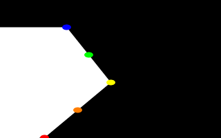
A simple "Spline Workshop".

Now, we take a deep breath. We know that all looks a bit weird, but with some simple explanations, we can easily see what all this does.
First, we are using the orthographic camera. If we haven't read up on that yet, a quick summary is: it renders the scene flat, eliminating perspective distortion so that in a side view, the objects look like they were drawn on a piece of graph paper (like in the side view of a modeller or CAD package). There are several uses for this practical new type of camera, but here it is allowing us to see our lathe and cylinders edge on, so that what we see is almost like a cross section of the curve which makes the lathe, rather than the lathe itself. To further that effect, we eliminated shadowing with the ambient 1 finish, which of course also eliminates the need for lighting. We have also positioned this particular side view so that <0,0> appears at the lower left of our scene.
Next, we declared a set of points. We note that we used 3D vectors for these points rather than the 2D vectors we expect in a lathe. That's the exception we mentioned earlier. When we declare a 3D point, then use it in a lathe, the lathe only uses the first two components of the vector, and whatever is in the third component is simply ignored. This is handy here, since it makes this example possible.
Next we do two things with the declared points. First we use them to place small diameter cylinders at the locations of the points with the circular caps facing the camera. Then we re-use those same vectors to determine the lathe. Since trying to declare a 2D vector can have some odd results, and isn't really what our cylinder declarations need anyway, we can take advantage of the lathe's tendancy to ignore the third component by just setting the z-coordinate in these 3D vectors to zero.
The end result is: when we render this code, we see a white lathe against a black background showing us how the curve we've declared looks, and the circular ends of the cylinders show us where along the x-y-plane our control points are. In this case, it's very simple. The linear spline has been used so our curve is just straight lines zig-zagging between the points. We change the declarations of Red_Point and Blue_Point to read as follows (see file lathdem3.pov).
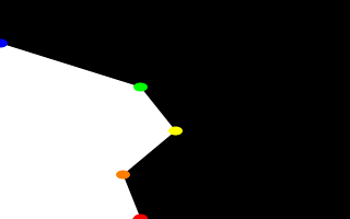
We re-render and, as we can see, all that happens is that the straight line segments just move to accomodate the new position of the red and blue points. Linear splines are so simple, we could manipulate them in our sleep, no?
Let's try something different. First, we change the points to the following (see file lathdem4.pov).
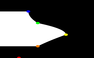
We then go down to the lathe declaration and change linear_spline to quadratic_spline. We re-render and what do we have? Well, there's a couple of things worthy of note this time. First, we will see that instead of straight lines we have smooth arcs connecting the points. These arcs are made from quadratic curves, so our lathe looks much more interesting this time. Also, Red_Point is no longer connected to the curve. What happened?
Well, while any two points can determine a straight line, it takes three to determine a quadratic curve. POV-Ray looks not only to the two points to be connected, but to the point immediately preceeding them to determine the formula of the quadratic curve that will be used to connect them. The problem comes in at the beginning of the curve. Beyond the first point in the curve there is no previous point. So we need to declare one. Therefore, when using a quadratic spline, we must remember that the first point we specify is only there so that POV-Ray can determine what curve to connect the first two points with. It will not show up as part of the actual curve.
There's just one more thing about this lathe example. Even though our curve is now put together with smooth curving lines, the transitions between those lines is... well, kind of choppy, no? This curve looks like the lines between each individual point have been terribly mismatched. Depending on what we are trying to make, this could be acceptable, or, we might long for a more smoothly curving shape. Fortunately, if the latter is true, we have another option.
The quadratic spline takes longer to render than a linear spline. The math is more complex. Still longer needs the cubic spline, yet, for a really smoothed out shape, this is the only way to go. We go back into our example, and simply replace quadratic_spline with cubic_spline (see file lathdem5.pov). We render one more time, and take a look at what we have.
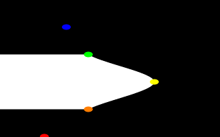
While a quadratic spline takes three points to determine the curve, a cubic needs four. So, as we might expect, Blue_Point has now dropped out of the curve, just as Red_Point did, as the first and last points of our curve are now only control points for shaping the curves between the remaining points. But look at the transition from Orange_Point to Yellow_Point and then back to Green_Point. Now, rather than looking mismatched, our curve segements look like one smoothly joined curve.
The concept of splines is a handy and necessary one, which will be seen again in the prism and polygon objects. But with a little tinkering we can quickly get a feel for working with them.
Almost every object can be approximated using triangles but we may need a lot of triangles to create more complex shapes. Thus we will only create a very simple mesh example. This example will show a very useful feature of the triangles meshes though: a different texture can be assigned to each triangle in the mesh.
Now let's begin. We will create a simple box with differently colored sides. We create an empty file called meshdemo.pov and add the following lines.
We must declare all textures we want to use inside the mesh before the mesh is created. Textures cannot be specified inside the mesh due to the poor memory performance that would result.
Now we add the mesh object. Three sides of the box will use individual textures while the other will use the global mesh texture.
Tracing the scene at 320x240 we will see that the top, right and front side of the box have different textures. Though this is not a very impressive example it shows what we can do with mesh objects. More complex examples, also using smooth triangles, can be found under the scene directory as chesmsh.pov and robotmsh.pov.
A polygon is defined by a number of points that describe its shape. Since polygons have to be closed the first point has to be repeated at the end of the point sequence.
In the following example we will create the word POV using just one polygon statement.
We start with thinking about the points we need to describe the desired shape. We want the letters to lie in the x-y-plane with the letter O being at the center. The letters extend from y=0 to y=1. Thus we get the following points for each letter (the z coordinate is automatically set to zero).
Letter P (outer polygon):
    <-0.8, 0.0>, <-0.8, 1.0>,
    <-0.3, 1.0>, <-0.3, 0.5>,
    <-0.7, 0.5>, <-0.7, 0.0>

Letter P (inner polygon):
    <-0.7, 0.6>, <-0.7, 0.9>,
    <-0.4, 0.9>, <-0.4, 0.6>

Letter O (outer polygon):
    <-0.25, 0.0>, <-0.25, 1.0>,
    < 0.25, 1.0>, < 0.25, 0.0>

Letter O (inner polygon):
    <-0.15, 0.1>, <-0.15, 0.9>,
    < 0.15, 0.9>, < 0.15, 0.1>

Letter V:
    <0.45, 0.0>, <0.30, 1.0>,
    <0.40, 1.0>, <0.55, 0.1>,
    <0.70, 1.0>, <0.80, 1.0>,
    <0.65, 0.0>
Both letters P and O have a hole while the letter V consists of only one polygon. We'll start with the letter V because it is easier to define than the other two letters.
We create a new file called polygdem.pov and add the following text.
As noted above the polygon has to be closed by appending the first point to the point sequence. A closed polygon is always defined by a sequence of points that ends when a point is the same as the first point.
After we have created the letter V we'll continue with the letter P. Since it has a hole we have to find a way of cutting this hole into the basic shape. This is quite easy. We just define the outer shape of the letter P, which is a closed polygon, and add the sequence of points that describes the hole, which is also a closed polygon. That's all we have to do. There'll be a hole where both polygons overlap.
In general we will get holes whenever an even number of sub-polygons inside a single polygon statement overlap. A sub-polygon is defined by a closed sequence of points.
The letter P consists of two sub-polygons, one for the outer shape and one for the hole. Since the hole polygon overlaps the outer shape polygon we'll get a hole.
After we have understood how multiple sub-polygons in a single polygon statement work, it is quite easy to add the missing O letter.
Finally, we get the complete word POV.

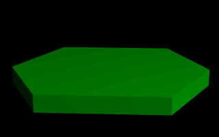
This produces a hexagonal polygon, which is then swept from y=0 through y=1. In other words, we now have an extruded hexagon. One point to note is that although this is a six sided figure, we have used a total of seven points. That is because the polygon is supposed to be a closed shape, which we do here by making the final point the same as the first. Technically, with linear polygons, if we didn't do this, POV-Ray would automatically join the two ends with a line to force it to close, although a warning would be issued. However, this only works with linear splines, so we mustn't get too casual about those warning messages!